Chapter 11Neural Language Models

The same task, different machinery

Chapter 10 left the n-gram model with two admitted blindnesses.

It cannot see far enough back. The Markov assumption throws away everything before the last $n-1$ words.

It cannot see that two words are related. To a counter, cat and dog are just different strings. A context seen with one lends no strength to the same context seen with the other.

This chapter repairs the second. The chapter after it repairs the first.

The task does not change by a single symbol. We still want $p(w_i \mid w_{i-n+1}, \ldots, w_{i-1})$. We still train by maximum likelihood. We still measure ourselves with the perplexity of Section that section. Only the apparatus that produces the probability is replaced.

Why counting cannot share strength

The fix follows from the diagnosis, so the diagnosis is worth stating carefully.

A trigram model over $|V| = 10{,}000$ words has one free number for every possible three word cell. That is about $10^{12}$ of them, as Equation (10.7) counted.

No corpus fills more than a vanishing fraction. Worse, the cells are entirely independent of one another.

Learning $p(\text{barked} \mid \text{the dog})$ tells the model nothing whatsoever about $p(\text{barked} \mid \text{the puppy})$. The two are different cells, and the table has no notion that dog and puppy are neighbours.

The founding idea of neural language modelling, due to , is to stop storing a number per context. Instead, compute the probability from a learned dense representation of each word.

Those are the distributed representations of Chapter 9. Similar words get similar vectors, and therefore, automatically, similar predictions.

The architecture

Fix a context of the previous $n-1$ words. The model computes the distribution over the next word in four movements. Each one is machinery from Chapter 8.

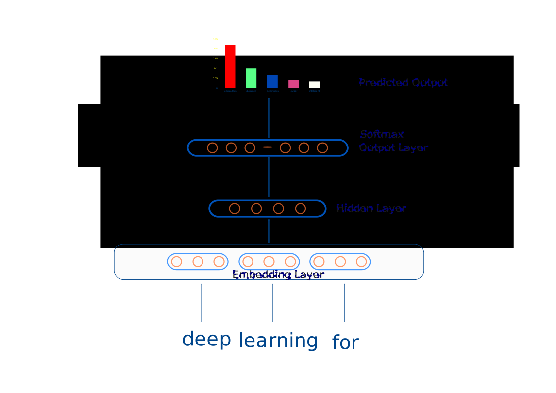
Look up.

Every word $w$ owns a row of an embedding matrix $E \in \mathbb{R}^{|V| \times d}$. The row $E_w$ is its dense vector.

The one-hot index of a context word selects its row. That is a lookup, not a multiplication, though it is convenient to write it as multiplying a one-hot vector by $E$.

The same matrix $E$ serves every context position. This sharing is the whole point of the chapter.

Concatenate.

The $n-1$ context embeddings are strung together into one vector

$$x \;=\; [\,E_{w_{i-n+1}}; \ldots; E_{w_{i-1}}\,] \qquad \text{of length } (n-1)\,d .$$

This is the model’s entire memory of the past. Note that its length is fixed the moment $n$ is chosen. That fact returns at the end of the chapter.

Mix.

A hidden layer applies a learned affine map and a non-linearity:

$$\begin{equation} h \;=\; \tanh\!\big(W_h\,x + b_h\big), \qquad h \in \mathbb{R}^{H}. \label{eq:nnlm-hidden} \quad\text{(11.1)} \end{equation}$$

This lets the model form non-linear combinations of the context. It is where “the of” can learn to behave differently from the sum of its parts.

Score and normalise.

An output map produces one score per vocabulary word, and a softmax turns the scores into a distribution:

$$\begin{equation} \hat{y} \;=\; \operatorname{softmax}\!\big(W_o\,h + b_o\big), \qquad \hat{y}_k \;=\; \frac{\exp\big((W_o h + b_o)_k\big)} {\sum_{j=1}^{|V|} \exp\big((W_o h + b_o)_j\big)}. \label{eq:nnlm-softmax} \quad\text{(11.2)} \end{equation}$$

The entry $\hat{y}_k$ is the model’s estimate of $p(w_i = k \mid \text{context})$.

The parameters are $E$, $W_h$, $b_h$, $W_o$ and $b_o$. They are learned jointly, and $E$ is learned along with the rest.

Where the parameters live

A hand count is clarifying, and it explains much of what the field did next.

Take a modest configuration. Vocabulary $|V| = 10{,}000$, embedding dimension $d = 50$, a context of $n-1 = 3$ words, and a hidden layer of $H = 100$ units.

Two lessons fall out of that table.

First, compare the total against the trigram table. The counter needed about $10^{12}$ cells. The network needs $1.5$ million, which is $655{,}000$ times fewer, or almost six orders of magnitude.

And the network shares them. What the model learns about dog is available in every context where dog appears. A count table shares nothing between cells.

Second, look at the share column. Two thirds of the parameters sit in $W_o$, whose size is $H \times |V|$ and therefore grows with the vocabulary.

Every training step must compute the softmax denominator in Equation (11.2), a sum over all $|V|$ words. That output softmax is the computational bottleneck of neural language modelling.

The tricks for dodging it are already familiar. Hierarchical softmax , noise-contrastive estimation, and the negative sampling of Chapter 9 all exist for this reason.

Training: the same loss, learned representations

Training is maximum likelihood, exactly as before. The knob we turn is now the network’s weights rather than a table of counts.

The lectures derive the loss from first principles, and the derivation is short enough to give in full.

Write $\hat{y} = p(y \mid \text{context})$. For a single binary outcome this is a Bernoulli distribution, so

$$\begin{equation} p(y \mid \text{context}) \;=\; \hat{y}^{\,y}\,(1 - \hat{y})^{1-y}. \label{eq:bernoulli} \quad\text{(11.3)} \end{equation}$$

Take logs of Equation (11.3):

$$\begin{equation} \log p(y \mid \text{context}) \;=\; y \log \hat{y} \;+\; (1-y)\log(1 - \hat{y}). \label{eq:logbernoulli} \quad\text{(11.4)} \end{equation}$$

Maximising a log likelihood is minimising its negative, which gives the cross-entropy loss:

$$\begin{equation} \mathcal{E} \;=\; -\,y \log \hat{y} \;-\; (1-y)\log(1 - \hat{y}). \label{eq:nnlm-bce} \quad\text{(11.5)} \end{equation}$$

Our case is not binary but $|V|$-way, and the true target is a one-hot vector. So the sum runs over the vocabulary:

$$\begin{equation} \mathcal{L} \;=\; -\sum_{k=1}^{|V|} y_k \log \hat{y}_k \;=\; -\log \hat{y}_{\,k^\star}, \label{eq:nnlm-ce} \quad\text{(11.6)} \end{equation}$$

where $k^\star$ indexes the word that actually occurred. Because $y$ is one-hot, every term but one vanishes.

So the loss on one example is simply the negative log probability the model gave to the right answer.

Average Equation (11.6) over the corpus, take base two, and exponentiate. That is the perplexity of Section that section. Minimising cross-entropy and minimising perplexity are one objective in two sets of clothes.

Backpropagation sends the gradient of Equation (11.6) back through the softmax, through the hidden layer, and into $E$ itself. The word vectors are not given to the model. They are learned, as a by-product of learning to predict.

One forward pass, every number shown

Take a model small enough to print. Vocabulary of five words, $d = 2$, $H = 3$, context of two words. The context is the cat and the target is sat.

Look up and concatenate:

$$E_{\text{the}} = (0.20,\, -0.10), \quad E_{\text{cat}} = (0.80,\, 0.30), \quad x = (0.20,\, -0.10,\, 0.80,\, 0.30).$$

Mix through Equation (11.1), then score and normalise through Equation (11.2).

The target received $0.1865$. So by Equation (11.6) the loss is $-\log(0.1865)$, which is $1.6794$ nats.

A model scoring every token this way would have perplexity $5.36$, against a vocabulary of five.

That is a model doing no better than guessing, which is correct. It has not been trained yet.

One backward pass

The gradient at the output layer is $\hat{y} - y$, the same prediction-minus-target that appeared in Chapter 9.

One step of gradient descent with $\eta = 0.5$ moves every parameter, including the two context rows of $E$:

$$\begin{aligned} E_{\text{the}} &: (0.200,\, -0.100) \;\to\; (0.223,\, -0.050), \\ E_{\text{cat}} &: (0.800,\, 0.300) \;\to\; (0.740,\, 0.325). \end{aligned}$$

And the prediction improves.

The loss fell from $1.6794$ to $1.1362$. Repeat a few million times and you have a language model.

Does it actually generalise?

The claim so far is that shared representations let the model handle word combinations it never saw. That claim is testable, so we should test it.

A corpus with something to learn

Build two families. Five pets rest in four indoor places. Five farm animals rest in four outdoor places.

Every sentence has the form “the ANIMAL rests PLACE”, and each animal is only ever paired inside its own family. That gives $40$ sentences.

The animal sits inside the trigram context, so a counter can see it too. Nothing is hidden from the baseline.

Hold out $8$ sentences. Keep $6$ more for deciding when to stop training. Train on the remaining $26$. Score only the place slot, since the place is what the animal is supposed to determine.

The first attempt fails

Train the network and watch both perplexities.

Training perplexity falls the whole way and never looks back. Held-out perplexity bottoms early and then climbs by a factor of more than ten.

The model has stopped learning the pattern and started memorising the pairs it was given. This is overfitting, and a network with more parameters than training examples will do it every time.

The remedy is the third split. Watch perplexity on the development set and keep the weights from its best moment. That is early stopping, and it is why a project needs three splits rather than two.

The second attempt

With early stopping in place, run six random splits.

The neural model wins on every split, by an overall factor of $4.55$.

The trigram model sits near $40$ because a held-out pair is a cell it never counted. It falls back to the smoothing floor, which is nearly uniform over the places. The network does not fall back. It computes.

Why it works, and a surprise

Nobody told the model that kitten resembles cat, or that a sofa is not a meadow. Two matrices hold what it worked out. $E$ is where a word goes in. $W_o$ is where a word comes out.

Read the two columns separately, because they disagree.

In $E$ the animals separate cleanly. Cat and puppy score $+0.783$ while cat and horse score $-0.336$. The places do not separate at all. Sofa and cushion reach $+0.271$ against sofa and meadow at $+0.225$, which is no distinction.

In $W_o$ it is the exact reverse. The places separate, $+0.650$ against $-0.051$ on those same two pairs. The animals stop separating, with cat and horse reaching $+0.652$.

The cause is the template. An animal only ever appears as context, so only its row of $E$ is trained. A place only ever appears as a target, so only its column of $W_o$ is trained. Each word learned its structure in exactly the matrix it was used in.

That explains a design choice from two chapters ago. It is why word2vec keeps two vectors per word, and why GloVe keeps $w$ and $\tilde{w}$. Being a context and being a target are different jobs, and one vector cannot hold both.

The generalisation now follows. A held-out animal lands near an animal the model has seen, so its prediction transfers. A count table has no such geometry, and every unseen pair drops to the floor.

Try it yourself. code/worked_examples/neural_lm.py produces every table in this chapter. --params prints the parameter breakdown, --forward the forward and backward pass, and --generalise runs the whole experiment, including the overfitting curve and the two cosine columns. Add --seeds 10 to check that the result is not luck.

Run it in ColabNotebookSource

The log-bilinear bridge

Between the count-based world and the fully neural one sits a model clean enough to deserve its own section.

Strip the hidden non-linearity of Equation (11.1) away entirely. Predict a single target feature vector by a linear combination of the context embeddings, $\hat{r} = \sum_{k} C_k\,E_{w_k}$. Then score each candidate word by how well its own embedding matches that prediction:

$$\begin{equation} p(w_i = k \mid \text{context}) \;=\; \frac{\exp\!\big(\hat{r}^{\top} E_k + b_k\big)} {\sum_{j=1}^{|V|} \exp\!\big(\hat{r}^{\top} E_j + b_j\big)}. \label{eq:lbm} \quad\text{(11.7)} \end{equation}$$

This is the log-bilinear model of . It has no hidden layer and no non-linearity, and it still beat n-gram models on perplexity.

That result carries an argument. The gain came from shared representations, not from depth.

Two of its details are quietly illuminating. The per-word bias $b_k$ ends up encoding roughly the unigram log frequency of word $k$, so the model reconstructs the frequency prior for free. That is the same job GloVe’s biases did in Chapter 9.

And Equation (11.7) is a dot product between a context vector and a word vector, followed by a softmax. That is the skip-gram objective seen from another angle.

So the embeddings of Chapter 9 and the language models of this chapter are the same machine with two emphases. word2vec cares about the vectors and treats prediction as a means. The language model cares about the prediction and treats the vectors as a means. Both fall out together.

What is fixed, and what is not

The representation gap is closed. Words that behave alike acquire vectors that sit alike. Prediction is computed rather than looked up, and generalisation to unseen combinations is now measurable.

On the first blindness of Chapter 10 the model has made no progress at all, and one line of the architecture already said why.

The context is a fixed-length concatenation of exactly $n-1$ embeddings. Choosing $n$ freezes the window as rigidly as it was frozen for the counter.

A neural 4-gram model sees three words of history and not one word more. Everything before falls off the same cliff.

Take “the book that the committee rejected was short”. The subject sits eight words back. No window of three can reach it, however rich the embeddings inside that window are.

The lectures list the consequences, and they are worth naming as a group.

The model is memoryless. It does not know where the context came from or what preceded it.

It cannot accept arbitrary input length. The architecture is fixed the moment the window is chosen.

Every context is treated in isolation. Nothing carries from one prediction to the next.

It is not a state machine. Many language tasks need a summary of the whole sentence, and this model has nowhere to keep one.

Temporal dependencies are therefore lost. If a word occurs twice in a sentence and the window cannot span both, the model learns it twice as if they were unrelated.

Towards sequence learning

What we need is an architecture with no fixed limit on the prior context. One that reads left to right, carrying a summary of everything seen so far and updating it at each word.

That summary is a state. The update rule is a recurrence. The model that results is the recurrent neural network of Chapter 12.

It keeps every gain of this chapter. The shared embeddings, the softmax head, the cross-entropy objective and the perplexity yardstick all carry over untouched. Only the window finally goes.

Further reading.

is the founding paper of neural language modelling and remains readable. introduce the log-bilinear family. give the hierarchical softmax that first made the output layer affordable. present the same lookup, concatenate, mix and softmax structure used here.