Chapter 9Learned Word Embeddings

From counting to learning

Part II opened with the distributional hypothesis. Firth’s slogan that “you shall know a word by the company it keeps”. We turned it into geometry by counting co-occurrences and reducing the matrix with an SVD.

Those count based vectors work. They also carry the whole matrix’s baggage. They are large, they are sparse, and they must be rebuilt from scratch whenever the corpus changes.

Around 2013 a different idea took over, and every modern system inherits it. Do not count contexts and then compress. Learn a small dense vector for each word directly, by training a model to predict context.

The distributional hypothesis is unchanged. Only the machinery is new. That machinery turns out to be faster and smaller, and it produces geometry with structure nobody put there on purpose.

word2vec

The canonical method is word2vec, from Mikolov and colleagues in 2013. It trains vectors through a deliberately trivial prediction task.

There are two formulations, and they are mirror images.

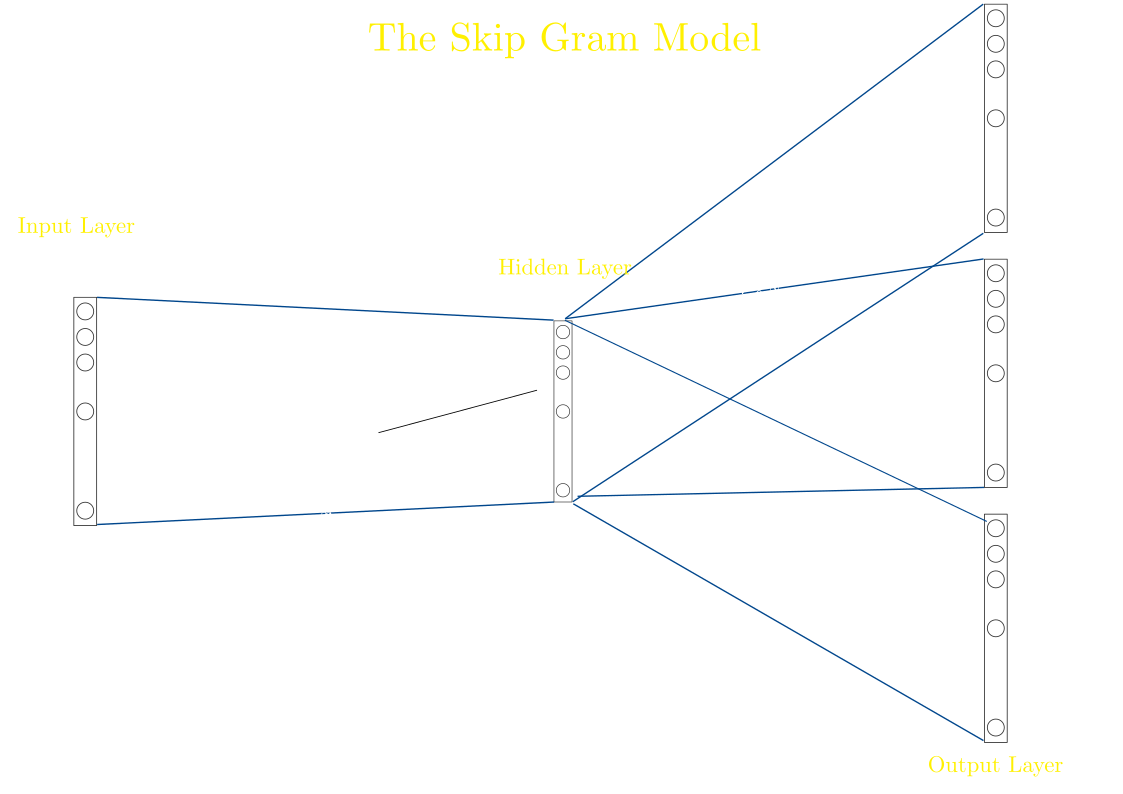
Skip-gram

Slide a window across the corpus. Take the word at the centre. Try to predict each of the words around it, one at a time.

That is the entire supervised signal. Centre word in, one context word out. No labels are needed, because the corpus labels itself.

Formally, for a corpus $w_1, \ldots, w_T$ and a window of $C$ words on each side, skip-gram maximises

$$\begin{equation} \frac{1}{T}\sum_{t=1}^{T} \sum_{\substack{-C \le c \le C \\ c \neq 0}} \log P(w_{t+c} \mid w_t). \label{eq:skipgram-objective} \quad\text{(9.1)} \end{equation}$$

CBOW

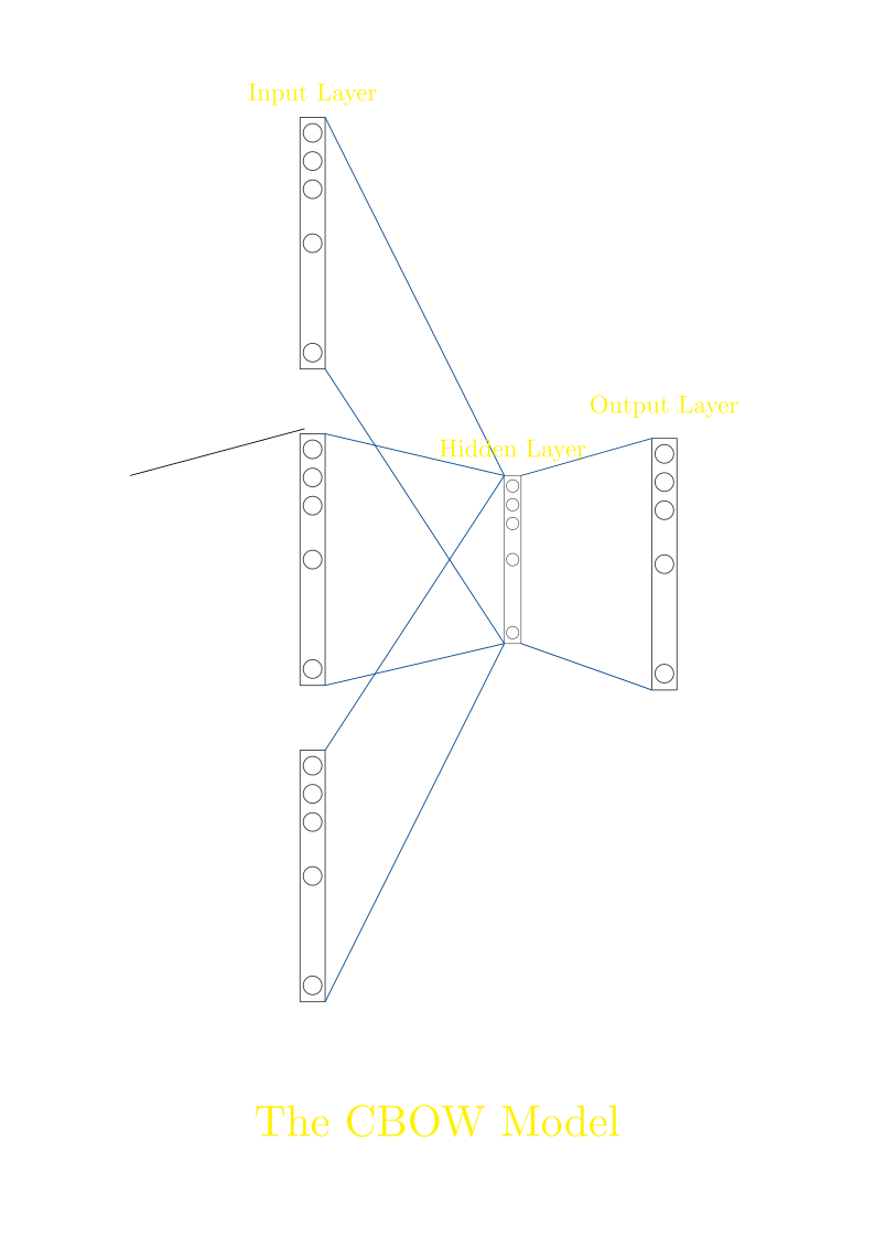
CBOW, for continuous bag of words, reverses every arrow. Take the surrounding words and predict the one in the middle.

The context words are combined before they reach the hidden layer, and the combination is a simple average:

$$\begin{equation} h \;=\; \frac{1}{2C}\sum_{\substack{-C \le c \le C \\ c \neq 0}} v_{w_{t+c}} . \label{eq:cbow-hidden} \quad\text{(9.2)} \end{equation}$$

That average is where the name comes from. The context is a bag. Order inside the window is discarded, so the cat sat and sat cat the give the same hidden vector.

The same sentence, both ways

Take “the quick brown fox jumps” with a window of two words on each side. Both formulations see the same windows and make different training data from them.

The counts differ, and that difference explains everything else about the two.

Skip-gram produces 14 training pairs from this one sentence, one per centre and context combination. CBOW produces 5, one per centre word.

Which to use

The averaging in Equation (9.2) is what costs CBOW its accuracy on rare words. A rare word in a context of four is one quarter of one hidden vector. The three common words beside it smooth its contribution away.

Skip-gram gives that rare word its own training pair with every neighbour, so it gets $2C$ chances to shape its own vector. It pays for this in time. More pairs means more updates.

The rule of thumb: CBOW for large corpora where speed matters, skip-gram when the tail matters.

What the model actually holds

The model has almost no parameters. One vector per word, or strictly two.

Every word $w$ has an input vector $v_w$, a row of $W$, used when $w$ is the centre or context being fed in. It also has an output vector $v'_w$, a column of $W'$, used when $w$ is the word being predicted.

Training nudges those vectors so words appearing in similar contexts end up with similar vectors. When training finishes the output vectors are usually thrown away, and the input matrix $W$ is what people mean by “the embeddings”.

The network, written out

word2vec is a neural network with one hidden layer and no nonlinearity in it. Writing it out properly takes four steps.

Let the vocabulary be size $V$ and the embedding size $N$. There are two weight matrices. $W$ is $V \times N$ and holds the input vectors. $W'$ is $N \times V$ and holds the output, or context, vectors.

Step 1: the hidden layer is a lookup.

The input $x$ is one hot for the centre word $w_I$. So

$$\begin{equation} h \;=\; W^{\!\top} x \;=\; v_{w_I}, \label{eq:w2v-hidden} \quad\text{(9.3)} \end{equation}$$

which is just row $w_I$ of $W$. No arithmetic happens here. Multiplying a one hot vector by a matrix selects a row, and that row is the word’s embedding.

Step 2: score every word.

For each candidate output word $w_j$, take the dot product of the hidden vector with that word’s context vector:

$$\begin{equation} u_j \;=\; {v'_{w_j}}^{\!\top} h . \label{eq:w2v-score} \quad\text{(9.4)} \end{equation}$$

Step 3: softmax.

Turn the $V$ scores into a distribution:

$$\begin{equation} y_j \;=\; \frac{\exp(u_j)}{\sum_{j'=1}^{V} \exp(u_{j'})} \;=\; \frac{\exp\!\big({v'_{w_j}}^{\!\top} v_{w_I}\big)} {\sum_{j'=1}^{V} \exp\!\big({v'_{w_{j'}}}^{\!\top} v_{w_I}\big)} . \label{eq:w2v-softmax} \quad\text{(9.5)} \end{equation}$$

Step 4: the loss.

We want to maximise the probability of the true context word $w_{j^*}$, so we minimise its negative log probability. That is cross entropy against a one hot target:

$$\begin{equation} E \;=\; -\log y_{j^*} \;=\; -u_{j^*} + \log \sum_{j=1}^{V} \exp(u_j). \label{eq:w2v-loss} \quad\text{(9.6)} \end{equation}$$

The two terms pull in opposite directions. Push up the score of the right word. Push down the total of all scores.

The gradients

Everything now follows from the chain rule, and the first derivative is the one you already know from Chapter 8.

Let $t_j$ be the target, $1$ for the true context word and $0$ otherwise. Differentiating Equation (9.6) gives the prediction minus target rule again:

$$\begin{equation} \frac{\partial E}{\partial u_j} \;=\; y_j - t_j \;=\; e_j . \label{eq:w2v-error} \quad\text{(9.7)} \end{equation}$$

That $e_j$ is the error at output unit $j$. Every remaining gradient is $e_j$ multiplied by whatever it was attached to.

Two consequences follow.

The output gradient $e_j h_i$ touches every word in the vocabulary, because $e_j$ is nonzero for all $j$. That is the cost we are about to attack.

The input gradient is multiplied by $x_k$, which is one hot. So only one row of $W$ moves per training example. The centre word’s embedding is updated and no other.

The obstacle

Now count the work. Equation (9.5) has a denominator summing over the whole vocabulary, and Equation (9.7) produces an error for every one of those words.

With $V$ in the hundreds of thousands, and billions of training examples, this is ruinous. Both fixes below attack the same denominator.

Hierarchical softmax

The first fix changes the shape of the output layer. Instead of $V$ independent output units, build a binary tree whose leaves are the words.

Reaching any word in a balanced tree takes $\log_2 V$ decisions. For a million words that is about twenty steps rather than a million.

Each internal node $n$ carries its own vector $v'_n$. There are no output vectors for words at all any more, only for the nodes on the way to them.

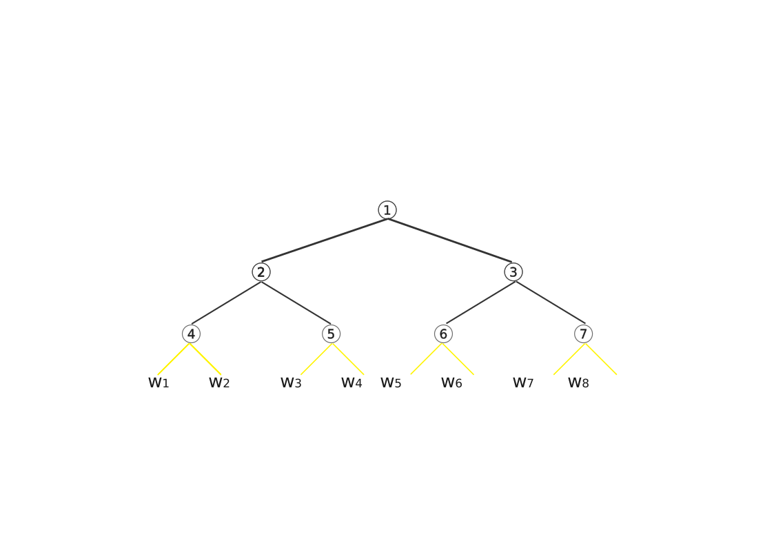
Write $L(w)$ for the number of nodes on the path from the root to word $w$. Write $n(w, j)$ for the $j$th node on that path. Then

$$\begin{equation} P(w \mid w_I) \;=\; \prod_{j=1}^{L(w)-1} \sigma\!\Big( \llbracket x_j \rrbracket \cdot {v'_{n(w,j)}}^{\!\top} h \Big), \label{eq:hsoftmax} \quad\text{(9.8)} \end{equation}$$

where the indicator is

$$\begin{equation} \llbracket x_j \rrbracket = \begin{cases} +1, & \text{if } n(w, j{+}1) \text{ is the } \mathit{left} \text{ child of } n(w,j) \\ -1, & \text{if it is the } \mathit{right} \text{ child.} \end{cases} \label{eq:hsoftmax-indicator} \quad\text{(9.9)} \end{equation}$$

The whole construction rests on one identity:

$$\begin{equation} \sigma(z) + \sigma(-z) = 1, \qquad\text{because}\qquad 1 - \sigma(z) = \sigma(-z). \label{eq:sigmoid-identity} \quad\text{(9.10)} \end{equation}$$

At every node the probability of going left and the probability of going right sum to one. So the probabilities of all $V$ leaves sum to one automatically. We get a proper distribution without ever computing a normalising sum.

A path worked out.

Take $V = 8$ and a balanced tree of depth 3. Suppose the path to cat goes left, then right, then left, and the hidden vector is $h = (0.5, -0.2)$.

Multiply the three: $P(\mathit{cat} \mid w_I) = 0.5449 \times 0.5622 \times 0.5646 = \mathbf{0.1730}$.

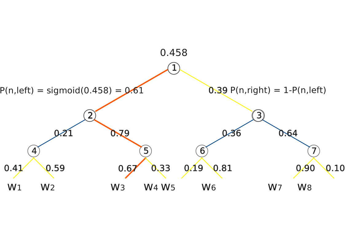
Three sigmoid evaluations replaced a softmax over eight words. Check the identity at the first node: $\sigma(+0.180) = 0.5449$ and $\sigma(-0.180) = 0.4551$, which sum to exactly $1$.

Its loss and gradients.

The loss is the negative log of Equation (9.8):

$$\begin{equation} E \;=\; -\sum_{j=1}^{L(w)-1} \log \sigma\!\big(\llbracket x_j \rrbracket u_j\big), \qquad u_j = {v'_{n(w,j)}}^{\!\top} h . \label{eq:hsoftmax-loss} \quad\text{(9.11)} \end{equation}$$

For the path above, $E = -\log(0.1730) = 1.7547$.

Differentiating gives a familiar shape:

$$\begin{align} \frac{\partial E}{\partial u_j} &= \big(\sigma(\llbracket x_j \rrbracket u_j) - 1\big)\, \llbracket x_j \rrbracket \label{eq:hsoftmax-grad-u} \\ \frac{\partial E}{\partial v'_j} &= \big(\sigma(\llbracket x_j \rrbracket u_j) - 1\big)\, \llbracket x_j \rrbracket \cdot h \label{eq:hsoftmax-grad-v} \\ \frac{\partial E}{\partial h} &= \sum_{j=1}^{L(w)-1} \big(\sigma(\llbracket x_j \rrbracket u_j) - 1\big)\, \llbracket x_j \rrbracket \cdot v'_j \label{eq:hsoftmax-grad-h} \end{align}$$

and the centre word is updated with $v_{w_I} \leftarrow v_{w_I} - \eta\,\partial E / \partial h$.

Only the $\log_2 V$ nodes on the path are touched. Every other node in the tree is left alone.

In practice the tree is a Huffman tree, built from word frequencies. Frequent words then sit on short paths and cost least to compute.

Negative sampling

The output layer is the problem. Predicting a context word means a softmax over the entire vocabulary. With a vocabulary in the hundreds of thousands, computing that denominator for every training example is ruinous.

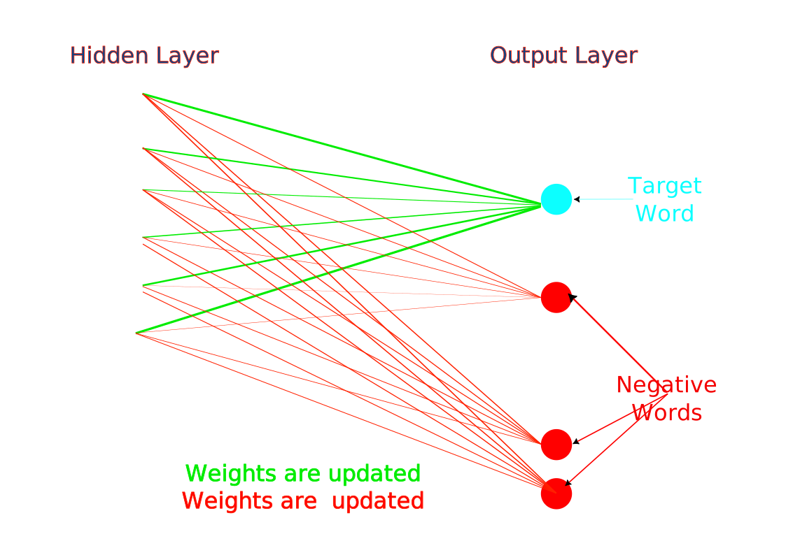
word2vec’s decisive trick is negative sampling. Do not ask which of all $V$ words is the context. Ask a handful of much easier yes or no questions.

Is this the real context word? Yes. Is this randomly drawn word? No, it is a negative.

Train the vectors to say yes to true pairs and no to a few random ones. A $V$-way softmax becomes a handful of binary decisions per example. That is what made word2vec fast enough to train on billions of words on one machine.

Where the 0.75 comes from

Chapter 7 promised this exponent would return, so here it is.

The negatives are not drawn uniformly, and they are not drawn from the raw unigram distribution either. They come from the unigram counts raised to the power $0.75$:

$$\begin{equation} q(w) \;=\; \frac{\operatorname{count}(w)^{0.75}} {\sum_{w'} \operatorname{count}(w')^{0.75}}. \label{eq:negsampling-dist} \quad\text{(9.12)} \end{equation}$$

Why bend the distribution at all? Draw negatives from the raw counts and nearly every negative is the, which teaches the model almost nothing. Draw them uniformly and rare words appear as negatives far more often than they ever appear as real words.

The $0.75$ power sits between the two. Here is what it does to a five word vocabulary.

In the last column, the most frequent word is sampled slightly less than its share, and the rarest more than four times its share. Raising counts to a power below one compresses the range, which lifts the tail and trims the head.

The same exponent did the same job for PMI in Chapter 7. There it smoothed the context distribution, to stop rare words earning inflated scores. Two methods, one correction, and no coincidence. word2vec can be shown to be implicitly factorising a shifted PMI matrix.

One training step, by hand

The update is the prediction minus target rule from Chapter 8, applied to a dot product. Nothing new is needed.

Take a centre word cat with vector $v = (0.5, -0.2)$. Take the true context word sat with vector $u^{+} = (0.4, 0.1)$, and one sampled negative the with $u^{-} = (-0.3, 0.6)$. The learning rate is $\eta = 0.1$.

For each pair the model scores $z = v \cdot u$, squashes it with a sigmoid, and compares with the label. The label is $1$ for the true context and $0$ for a negative.

The signs are the whole story. The positive pair gets a negative gradient, which pulls the two vectors together. The negative pair gets a positive one, which pushes them apart.

Now apply $u \leftarrow u - \eta\,(\sigma(z) - y)\,v$ to each context vector.

Did it work? Recompute both scores with the updated vectors.

True pairs pulled together, random pairs pushed apart. Repeat a few billion times and the geometry of Part II falls out.

Try it yourself. code/worked_examples/word2vec.py prints both tables above. --exponent lets you change the $0.75$ and watch the sampling distribution flatten or sharpen.

Run it in ColabNotebookSource

The negative sampling objective

Written out, the loss for one centre word with $k$ negatives is

$$\begin{equation} E \;=\; -\Big[\, \log \sigma(z_{\text{pos}}) \;+\; \sum_{i=1}^{k} \log\big(1 - \sigma(z_{\text{neg}_i})\big) \,\Big], \label{eq:negsampling-loss} \quad\text{(9.13)} \end{equation}$$

where $z = {v'_w}^{\!\top} h$ is the score of a candidate word.

Apply Equation (9.10) and the second term becomes $\sum_i \log \sigma(-z_{\text{neg}_i})$, which is the form usually printed. Both say the same thing. Make the true pair score high and the sampled pairs score low.

Compare this with the full softmax loss of Equation (9.6). The sum over $V$ has become a sum over $k$, and $k$ is typically 5 to 20.

What each fix costs

Put the three side by side. Let $T$ be the corpus size, $N$ the embedding dimension, and $C$ the window size.

For $V = 10^6$, the full softmax costs a million operations per prediction. Hierarchical softmax costs about twenty. Negative sampling costs $k$, and $k$ does not grow with the vocabulary at all.

Both fixes are approximations, and they approximate different things. Hierarchical softmax still computes a genuine probability distribution, just factored over a tree. Negative sampling abandons the distribution entirely and solves a set of binary classification problems instead. In practice negative sampling won, because it is simpler and trains faster on frequent words.

Negative sampling is a pattern this book meets again. Pull true pairs together, push random pairs apart. The contrastive training behind dense retrieval in Chapter 20 is the same idea one level up, with positive and negative pairs shaping a representation.

The analogy surprise

Something unplanned fell out of these vectors.

Take the vector for king. Subtract man. Add woman. The nearest vector to the result is queen.

The relationship from male to female turns out to be, approximately, a direction in the space. The same displacement carries uncle to aunt and he to she. Plural formation is another direction. Capital of country is another.

Nobody designed this. It emerged because consistent semantic relationships produce consistent contextual differences, and training recorded them as consistent geometric ones.

Analogy solving becomes arithmetic:

$$\begin{equation} \text{analogy}(a, b, c) \;=\; \operatorname*{nearest}\big(v_b - v_a + v_c\big), \label{eq:analogy} \quad\text{(9.14)} \end{equation}$$

excluding $a$, $b$ and $c$ themselves from the answer.

The analogy worked out

Take a toy space with three interpretable dimensions: how royal a word is, how male, how female.

Compute the target. Subtracting man from king strips the male component and keeps the royal one. Adding woman puts a female component back:

$$v_{\mathit{king}} - v_{\mathit{man}} + v_{\mathit{woman}} = (1.00, 0.10, 0.90).$$

Now rank every word by cosine to that target.

Queen wins at $0.9991$, and the runners up are interpretable. Throne is royal but carries no gender. Prince is royal but male. Both are near, and both are wrong for the right reasons.

Note where woman lands: third, ahead of four other words. On real spaces a query word very often comes first, because $v_b - v_a + v_c$ stays close to $v_c$. Forget the exclusion and your analogy scores will look far better than they are. It is the single most common way to overstate an embedding.

Subtracting a direction: what apple is made of

The analogy above used a famous example on a space built to make it work. Here is a more honest use of the same arithmetic, and it doubles as a diagnosis of the corpus.

Take a space trained on technology news. Ask for the nearest neighbours of apple.

The top four are technology. The first fruit trails at $0.59$, and it is orange, which is a phone network as well as a fruit.

This tells us something about the corpus rather than about English. Apple is overwhelmingly a company here. The fruit sense exists in the vector, but it is buried under the company sense, because the training text talked about one far more than the other.

Now subtract the strongest technology association and see what is left:

$$\begin{equation} \vec{d} \;=\; \vec{\mathit{apple}} - \vec{\mathit{iphone}} . \label{eq:apple-minus-iphone} \quad\text{(9.15)} \end{equation}$$

Rank every word by cosine to $\vec{d}$.

The list has inverted completely. Fruits fill the top. The technology words have gone negative, meaning they now point away from what is left.

Nothing was told to the model about fruit or about companies. Subtracting one word removed a whole semantic dimension, and the sense that had been buried came to the surface.

Why this works.

A vector is a mixture of the senses and associations the corpus gave the word. Apple carries a large technology component and a smaller fruit one. Iphone carries the technology component and no fruit at all.

Subtracting cancels what they share and keeps what only the first has. The technology part very nearly annihilates, and the fruit part survives untouched. The residue is the minority sense.

What it is good for.

This is a practical diagnostic, and worth more than analogy scores.

It reveals the dominant sense of a polysemous word, which is a fact about your training data. If apple comes out as a company, your corpus is technology news. If it comes out as a fruit, your corpus is recipes or agriculture. The same probe on bank, java, python or amazon will tell you what your text was about before you read a line of it.

It also shows the limit of a single vector per word. Both senses are jammed into one point, and pulling them apart takes arithmetic and a guess about what to subtract. Chapter 15 solves this properly by letting the sentence decide which sense is present.

Try it yourself. code/worked_examples/word2vec.py --apple prints both tables. --subtract takes any word, so you can strip a different association and see what surfaces.

Run it in ColabNotebookSource

GloVe

word2vec learns from local windows, one at a time. It never sees the corpus as a whole. GloVe asks whether that is wasteful, given that the global co-occurrence counts are sitting right there.

Meaning lives in ratios

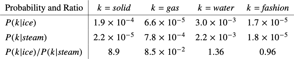
GloVe’s founding observation is not about counts. It is about ratios of counts.

Let $X_{ij}$ be the number of times word $j$ occurs in the context of word $i$. The conditional probability is

$$\begin{equation} P_{ij} \;=\; P(j \mid i) \;=\; \frac{X_{ij}}{\sum_k X_{ik}} . \label{eq:glove-prob} \quad\text{(9.16)} \end{equation}$$

Take a single probability such as $P(\mathit{solid} \mid \mathit{ice})$. It is hard to interpret. Is $0.00019$ large? There is nothing to compare it against.

Now take two words and probe them with a third. Compare $P(k \mid \mathit{ice})$ against $P(k \mid \mathit{steam})$ for various probe words $k$. The ratio is immediately readable.

The ratio is large when the probe belongs to the first word. It is small when the probe belongs to the second. It sits near one when the probe belongs to both, or to neither.

That is the discrimination raw probabilities could not give. Water and fashion both score near one, for opposite reasons, and the ratio quite properly refuses to distinguish them: neither tells ice from steam.

Turning a ratio into an objective

If ratios carry the meaning, the model should predict them. GloVe arranges for the dot product of two word vectors to approximate the log of the co-occurrence count, because differences of logs are ratios.

That gives a weighted least squares problem:

$$\begin{equation} J \;=\; \sum_{i,j=1}^{V} f(X_{ij}) \Big( w_i^{\!\top} \tilde{w}_j + b_i + \tilde{b}_j - \log X_{ij} \Big)^{2} . \label{eq:glove} \quad\text{(9.17)} \end{equation}$$

Each piece earns its place.

$w_i$ is the vector for the word, $\tilde{w}_j$ the vector for the context. Every word again gets two, exactly as word2vec has input and output vectors. The final embedding is usually $w + \tilde{w}$, since both carry signal.

The biases $b_i$ and $\tilde{b}_j$ absorb how common each word is on its own. Without them the model would have to encode raw frequency in the vectors, which is the pollution PMI existed to remove in Chapter 7.

The target is $\log X_{ij}$, not $X_{ij}$. A log turns the multiplicative structure of counts into an additive one, so a difference of dot products lands on a ratio of probabilities. That is the whole design.

The weighting function

The last piece is $f$, and without it the objective would be dominated by whichever pairs happen to be most frequent.

$$\begin{equation} f(x) \;=\; \begin{cases} (x / x_{\max})^{\alpha}, & x < x_{\max} \\ 1, & \text{otherwise,} \end{cases} \qquad \alpha = 0.75, \quad x_{\max} = 100 . \label{eq:glove-weight} \quad\text{(9.18)} \end{equation}$$

It does three jobs at once.

At $x = 0$ it gives $f(0) = 0$, so pairs that never co-occur contribute nothing. This matters, because $\log 0$ is undefined and most of the matrix is zeros.

Between $0$ and $x_{\max}$ it rises, so rarer pairs count less than common ones, which suppresses noise from pairs seen once or twice.

Above $x_{\max}$ it is flat at $1$. A pair seen ten thousand times gets no more weight than one seen a hundred times, so the cannot dominate the fit.

That exponent is $0.75$ for the third time in this book, after PMI smoothing and negative sampling. Three different models, three different mechanisms, and the same correction: compress the range so the head does not swamp the tail.

Where GloVe stands

At release in 2014 it beat the alternatives on three tasks: word analogy, word similarity and named entity recognition. It captured syntactic and semantic relationships equally well.

It shares word2vec’s fatal limitation, though. GloVe produces static embeddings, one vector per word, and contextual models have since displaced it for most tasks.

FastText

Both models so far treat a word as an atom. A word is either in the vocabulary with a vector of its own, or it is unknown and has nothing.

Chapter 3 showed why that fails. Heaps’ law guarantees the vocabulary never closes, so unknown words keep arriving forever.

FastText answers the same pressure that subword tokenisation answered in Chapter 5, but at the embedding rather than the tokeniser.

A word is a bag of character n-grams

Break each word into overlapping character n-grams. Mark the boundaries with < and >, so a prefix can be told from the same letters appearing mid-word.

For apple with $n = 3$:

FastText normally uses several values of $n$ together. Here is technical at $n = 3$ and $n = 4$.

Every n-gram gets its own learned vector $\mathbf{z}_g$. The word’s vector is their sum, and the whole word is included in the set as well:

$$\begin{equation} \mathbf{w} \;=\; \sum_{g \in G(w)} \mathbf{z}_g . \label{eq:fasttext} \quad\text{(9.19)} \end{equation}$$

Written out for our example,

$$\begin{equation} \mathbf{w}_{\mathit{technical}} \;=\; \mathbf{z}_{\texttt{<te}} + \mathbf{z}_{\texttt{tec}} + \mathbf{z}_{\texttt{ech}} + \cdots + \mathbf{z}_{\texttt{cal}} + \mathbf{z}_{\texttt{al>}} + \mathbf{z}_{\mathit{technical}} . \label{eq:fasttext-worked} \quad\text{(9.20)} \end{equation}$$

Everything else is skip-gram with negative sampling, unchanged. Only the definition of a word vector has moved.

What that buys

Unknown words get real vectors.

Meet technicality for the first time and FastText still produces something sensible. Its n-grams tec, ech, chn and nic were all trained on technical and its relatives, so the sum lands near them.

word2vec and GloVe can only return an unknown token here. FastText returns a vector in roughly the right neighbourhood.

Morphology comes free.

Walk, walks, walked and walking share most of their n-grams, so their vectors are close by construction rather than by luck.

This matters far more in some languages than in English. A morphologically rich language such as Tamil, Finnish or Turkish generates enormous numbers of inflected forms, most of them individually rare. Treating each as an unrelated atom wastes almost all the evidence. Sharing subword vectors pools it.

The cost.

The n-gram table is larger than a word table, and a word vector must be assembled at query time rather than looked up. FastText also cannot separate unrelated words that happen to share spelling. Nothing tells it that ear in earth has no connection to ear in hearing.

The idea outlives the model

FastText itself is little used now. Its central move is everywhere.

Every modern tokeniser builds its vocabulary from frequent character sequences rather than whole words. BPE in Chapter 5, WordPiece, SentencePiece. All of them answer the open vocabulary problem the same way, by composing rare things from common pieces.

FastText made that argument at the embedding layer first.

Counting and learning are the same thing

Part II has now built dense word vectors three separate times. Chapter 7 factored a PPMI matrix with an SVD. This chapter trained word2vec by gradient descent, then fitted GloVe to global counts.

Three methods, three chapters, three sets of vectors that behave alike. That is not a coincidence, and the reason is the most useful idea in Part II.

All three are matrix factorisations of the same co-occurrence statistics. They differ in which matrix, which loss and which optimiser. They do not differ in kind.

One shape, three fillings

Every method here produces two matrices. A word matrix $W$ of size $V \times d$, and a context matrix $C$ of the same size. Row $i$ of $W$ is the vector $w_i$. Row $j$ of $C$ is the context vector $c_j$.

Every method then asks the dot product of a word and a context to reproduce some association score:

$$\begin{equation} w_i^{\!\top} c_j \;\approx\; M_{ij}. \label{eq:factorisation} \quad\text{(9.21)} \end{equation}$$

That is the whole family. Choosing a method means choosing three things: the matrix $M$, the weight each cell carries, and how you solve for $W$ and $C$.

The middle column is the surprising one. Nothing in word2vec’s training loop mentions PMI. The next subsection shows why PMI turns up anyway.

What word2vec is really computing

Recall the negative sampling objective of Equation (9.13). Take one word and one context, and write $x = w^{\!\top} c$ for their dot product.

Over the whole corpus that pair is seen $\#(w,c)$ times as a real pair. It also turns up as a sampled negative. A word $w$ is the centre of $\#(w)$ windows, each draws $k$ negatives, and each negative is $c$ with probability $P(c)$. So the pair appears as a negative $k \cdot \#(w) \cdot P(c)$ times in expectation.

Collect the two contributions:

$$\begin{equation} \ell(x) \;=\; \#(w,c)\,\log \sigma(x) \;+\; k\,\#(w)\,P(c)\,\log \sigma(-x). \label{eq:sgns-local} \quad\text{(9.22)} \end{equation}$$

Now differentiate and set the result to zero. Using $\sigma'(x) = \sigma(x)\sigma(-x)$,

$$\begin{equation} \frac{\partial \ell}{\partial x} \;=\; \#(w,c)\big(1 - \sigma(x)\big) \;-\; k\,\#(w)\,P(c)\,\sigma(x) \;=\; 0 . \label{eq:sgns-stationary} \quad\text{(9.23)} \end{equation}$$

Write $a = \#(w,c)$ and $b = k\,\#(w)\,P(c)$. Then $\sigma(x) = a / (a + b)$, and since $\sigma(x) = e^{x} / (1 + e^{x})$, this gives $e^{x} = a/b$. Substituting $P(c) = \#(c) / |D|$, where $|D|$ is the number of pairs in the corpus:

$$\begin{equation} w^{\!\top} c \;=\; \log \frac{\#(w,c)\,|D|}{\#(w)\,\#(c)} \;-\; \log k \;=\; \operatorname{PMI}(w, c) \;-\; \log k . \label{eq:sgns-is-pmi} \quad\text{(9.24)} \end{equation}$$

This is the result of . The optimum of skip-gram with negative sampling is a PMI matrix, shifted down by $\log k$. Two hundred dimensions of gradient descent, and the answer was in Chapter 7 all along.

The shift has a plain reading. More negatives means a higher bar. With $k=5$ every entry moves down by $\log 5 \approx 1.609$, so a pair needs stronger evidence before its dot product goes positive.

Watching it happen.

The claim is checkable on the eight-word matrix of Chapter 7. Train the objective directly, then compare each learned dot product against $\operatorname{PMI} - \log k$.

Across all $32$ observed pairs the mean absolute difference is $0.0024$, with $k = 5$. The largest is $0.0074$. The network was never shown a PMI value.

What GloVe is really computing

GloVe looks like a different animal, because Equation (9.17) fits $\log X_{ij}$ rather than an association score. The biases close the gap.

Start from the definition of PMI and expand it in raw counts. Write $X_{i\cdot}$ for a row total, $X_{\cdot j}$ for a column total, and $X_{\cdot\cdot}$ for the grand total:

$$\begin{equation} \operatorname{PMI}(i, j) \;=\; \log X_{ij} \;-\; \log X_{i\cdot} \;-\; \log X_{\cdot j} \;+\; \log X_{\cdot\cdot} . \label{eq:pmi-expanded} \quad\text{(9.25)} \end{equation}$$

Now read GloVe’s objective again. It asks for $w_i^{\!\top}\tilde{w}_j = \log X_{ij} - b_i - \tilde{b}_j$. The two biases are free parameters, fitted from the data. Set

$$b_i = \log X_{i\cdot} - \tfrac{1}{2}\log X_{\cdot\cdot}, \qquad \tilde{b}_j = \log X_{\cdot j} - \tfrac{1}{2}\log X_{\cdot\cdot},$$

and the right hand side becomes exactly Equation (9.25). GloVe’s dot product is fitting PMI, up to whatever the biases absorb.

That is what the biases were introduced to do. The GloVe section justified them as removing raw frequency from the vectors. Equation (9.25) says what removing raw frequency means. It means subtracting a row effect and a column effect, which is the arithmetic PMI performs.

The fitted numbers agree. On the same eight-word matrix the bias rises with the word’s row total. Tracking that total is the only job it has.

So three chapters of machinery converge on one target. SVD fits PPMI. word2vec fits PMI shifted by $\log k$. GloVe fits PMI with the shift absorbed into two bias terms.

That also settles a puzzle from earlier. The exponent $0.75$ appears in PMI smoothing, in negative sampling and in GloVe’s weighting function. It is the same correction applied to the same statistic, three times over.

Where they genuinely differ

Sharing a target does not make three methods interchangeable. The differences sit in the two remaining columns of the table: how each cell is weighted, and what happens to the zeros.

Weighting first. The SVD minimises squared error over every cell equally. A pair seen once therefore counts as much as a pair seen ten thousand times. word2vec weights each pair by how often it occurred, since the objective sums over actual windows. GloVe states its weighting outright in $f(X_{ij})$, and can therefore tune it.

The zeros matter more, and they are easy to miss. Most of a co-occurrence matrix is zeros, and the three methods treat them in three different ways. PPMI writes an explicit $0$ and the SVD fits it like any other cell. word2vec never fits a zero cell directly. Negative sampling still drags it down, because an unseen pair is drawn as a negative and never as a positive. GloVe sets $f(0) = 0$ and drops those cells entirely.

A case where the difference bites.

Take the matrix from Chapter 7: four animal words, four vehicle words, and no shared context at all. Compress to two dimensions by each method, then ask for nearest neighbours.

Two methods get all four right. GloVe gets all four wrong, and it is not a training failure. Its fit to $\log X_{ij}$ is good, at a mean absolute error of $0.018$.

The explanation is the zeros. On this matrix every fact that separates an animal from a vehicle lives in a cell that is zero. GloVe drops those cells, so it is never shown a single piece of evidence that a dog is unlike a truck. The two groups are fitted on disjoint contexts, and nothing ties them together. Their relative positions are left to the initialiser.

Fill each zero with a count of $1$ and GloVe recovers all four. Real corpora have almost no structural zeros, because in a large enough corpus most pairs eventually co-occur once. That is why this never became a practical problem, and it is also why the toy exposes the mechanism so cleanly.

The remaining difference is cost. The SVD needs the whole matrix in memory and a full decomposition, which is cubic in the smaller dimension. word2vec needs only a stream of windows and never builds the matrix at all. That, rather than vector quality, is why the learned methods took over in 2013.

Why $d$ and $K$ are the same question

The factorisation view also settles what the embedding dimension means.

In the SVD picture the top singular values carry most of the semantic structure. Chapter 7 used their decay to choose $K$, through the contribution ratio of Equation (7.10).

word2vec’s hidden layer dimension $d$ plays the identical role. It is a budget for how many directions you are willing to keep. The lectures put it as a parallel between hidden units and significant eigenvalues.

Choosing $d$ is therefore the bias variance trade off in disguise. Too few dimensions and semantic information is lost. Too many and you fit noise.

This predicts something you can check. Raise $d$ past the number of significant singular values and it should buy little. In practice it does.

So the useful $d$ tends to land near the count of large singular values. That is what the scree plot of Chapter 7 was showing all along.

Try it yourself. code/worked_examples/factorisation.py produces every number in this section, on the matrix Chapter 7 already used. Run it plain for all four steps. --sgns --k 1 shows the shift vanishing when there is one negative, and --k 15 shows it growing. --compare prints the neighbour table above, and --compare --fill 1 removes the structural zeros and watches GloVe come back into line.

Run it in ColabNotebookSource

Reading the geometry

An embedding space is not a black box. It is an object you can interrogate, and learning to read one is a practitioner’s core skill.

Every question you can ask reduces to one operation, the cosine similarity of Chapter 4:

$$\begin{equation} \cos(u, v) \;=\; \frac{u \cdot v}{\lVert u \rVert\,\lVert v \rVert}. \label{eq:cosine} \quad\text{(9.26)} \end{equation}$$

It ranges from $1$ for the same direction, through $0$ for orthogonal, to $-1$ for opposite.

We use the angle rather than the raw dot product for a specific reason. Vector length in these spaces tracks word frequency more than meaning. Direction is where the semantics live.

From cosine, three tools follow.

Nearest neighbours are the words of highest cosine to a target, excluding the target itself. They reveal what a word means to the space. The neighbours of bank expose whether your corpus was about rivers or money.

Analogies, through Equation (9.14), probe whether a relationship is encoded as a clean direction.

Failures are as informative as successes. On a corpus of a few thousand documents many analogies return nonsense. The relationship was never witnessed often enough to become a stable direction. Knowing that a bad analogy usually means thin data, not a broken method, is exactly the forensic skill Project 3 trains.

Embeddings encode the corpus, all of it

The geometry records whatever the corpus contains, including its social regularities. The apple probe above was a mild instance. What follows is the same fact with higher stakes.

Suppose a body of text systematically places occupation words near one gender’s pronouns. The space will place them near that gender’s vector. No single sentence is biased. The aggregate association is real and measurable.

Measuring it needs only cosine. The tool is the Word Embedding Association Test . In the simplified form this course uses, it scores the differential association of target words $T$ with two attribute sets $A$ and $B$:

$$\begin{equation} s(T, A, B) \;=\; \frac{1}{|T|}\sum_{t \in T} \Big[\operatorname*{mean}_{a \in A}\cos(t, a) - \operatorname*{mean}_{b \in B}\cos(t, b)\Big]. \label{eq:weat} \quad\text{(9.27)} \end{equation}$$

A positive $s$ means the targets sit closer on average to set $A$. A negative $s$ means closer to $B$. The magnitude is the strength.

Point it at institutional against narrative vocabulary and it separates registers. Point it at gendered attributes and it exposes occupational stereotypes in web scale spaces.

The number is honest and it demands honesty back. Three cautions.

It measures the corpus, through the model. Change either and $s$ changes.

The word lists are a design choice. Report them with the score, or the score means nothing.

A near zero result means these lists do not separate. It does not mean the space is unbiased.

Any system built on these vectors inherits their associations silently. Search, screening, classification, all of it. That is why measuring them is not an ethical afterthought. It is part of knowing what you have built.

The limit that motivates everything after

For all their elegance, these embeddings share one fatal limitation. Each word gets exactly one vector, forever.

The bank of a river and the bank that holds money collapse into a single point. That point is the blurred average of both senses, and it is correct for neither.

A word’s meaning depends on its sentence. A lookup table cannot represent that, because it committed to the vector before the sentence existed.

Repairing this is the achievement of the contextual embeddings and transformers of Part IV. Let a word’s representation depend on its context.

The tools you build here do not go away. Cosine, nearest neighbours and association tests are exactly how those larger models are probed and audited. Learning to read a space by hand now is learning to read every space later.

Further reading.

introduce negative sampling. on GloVe and on FastText are the siblings. is the WEAT paper and a model of careful measurement. explains word2vec’s parameter updates step by step. extends the idea from words to whole sentences and documents. analyses the linear algebraic structure that lets a single vector encode several senses of a word. proves that negative sampling factorises a shifted PMI matrix, and shows that much of word2vec’s reported advantage over counting was down to hyperparameters rather than method.