Chapter 12Recurrent Networks

A window that will not close

Chapter 11 fixed one blindness and left the other in plain sight.

The feed-forward language model concatenates $n-1$ embeddings into a single vector. That vector is its whole memory, and its length is decided before training begins.

So the model reads a sentence through a slot of fixed width. Everything outside falls away, exactly as it did for the counter.

Consider “the book that the committee rejected was short”. The verb agrees with book, eight words back. A window of three cannot see it.

Widening the window is not a fix. The hidden matrix $W_h$ has shape $(n-1)d \times H$, so its size grows with every word you admit.

And no fixed width is ever wide enough. Sentences have no maximum length.

What we want is a model that reads left to right. One that keeps a running summary of everything so far, and updates it at each word.

The summary is a state. The update rule is a recurrence.

The recurrence

A recurrent neural network keeps a hidden state $h_t$ and rewrites it at every time step:

$$\begin{align} h_t &= \tanh\!\big(W\,x_t + U\,h_{t-1} + b_h\big), \label{eq:rnn-state}\\ \hat{y}_t &= \operatorname{softmax}\!\big(V\,h_t + b_y\big). \label{eq:rnn-out} \end{align}$$

Here $x_t$ is the embedding of the word read at step $t$, and $h_0$ is conventionally the zero vector.

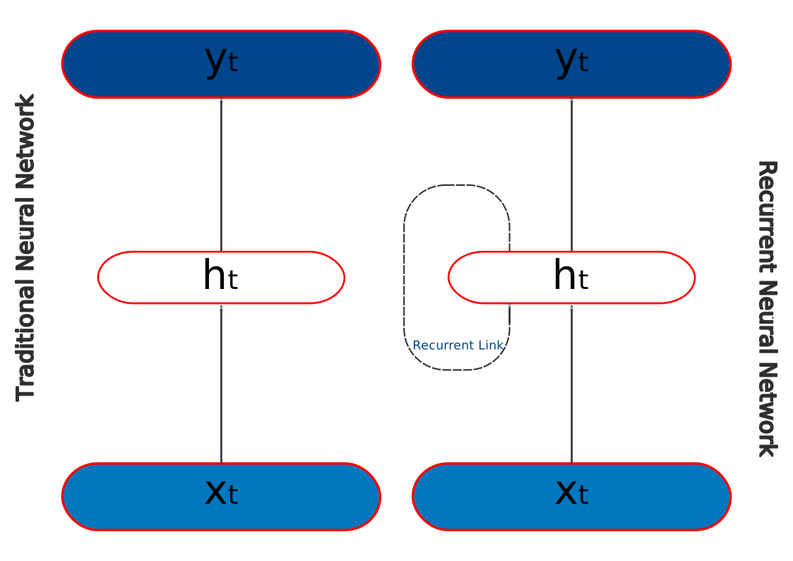
Three matrices carry the whole model.

$W$ maps the current word into the state. $U$ maps the previous state into the new one. $V$ maps the state to a score for every vocabulary word.

The important word is same. The same $W$, $U$ and $V$ are used at every step, however long the sentence. That reuse is what recurrent means.

Equation (12.8) therefore does something the feed-forward model could not. $h_{t-1}$ was itself computed from $h_{t-2}$, and so on back to the first word.

So the state at step $t$ depends on every word read so far. There is no window and no cliff.

Unrolling, worked

Take a model small enough to print. Two hidden units, embeddings of size two, a vocabulary of three words.

$$W = \begin{pmatrix} 0.6 & -0.3 \\ 0.2 & 0.5 \end{pmatrix}, \quad U = \begin{pmatrix} 0.4 & 0.1 \\ -0.2 & 0.7 \end{pmatrix}, \quad b_h = (0.05,\, -0.05).$$

Read the sentence the dog ran, starting from $h_0 = (0, 0)$.

Follow the third row. Its input column depends only on ran, but its $h_t$ depends on $h_2$, which depended on $h_1$, which depended on the.

So $h_3$ is a summary of the whole prefix. Nothing was thrown away, and no parameter was added to make room for it.

Why $\tanh$

The lectures ask why $\tanh$ rather than the sigmoid, and the answer is worth keeping.

$\tanh$ is symmetric about the origin, so its output is zero-centred. States that average to zero train faster than states that average to $0.5$.

Its derivative is also steeper. The sigmoid’s derivative lies in $[0, 0.25]$, while $\tanh$’s lies in $[0, 1]$.

A derivative capped at $0.25$ shrinks the gradient by at least a factor of four at every step. Section 1.5 shows why that is fatal, and $\tanh$ merely delays the problem rather than removing it.

Modern architectures mostly use ReLU and its variants, which pass gradient unchanged on the positive side. ReLU has its own failure: a unit whose input is always negative stops passing any gradient at all and never recovers. Leaky ReLU, $\max(\alpha x, x)$ with small $\alpha$, exists to prevent that.

An RNN is a language model

Equation (12.9) already produces one distribution over the vocabulary per time step, which is exactly what a language model needs.

Train it by predicting the next word at every position. The loss at step $t$ is the cross-entropy of Chapter 11, and the loss for a sentence is their sum:

$$\begin{equation} E_t \;=\; -\sum_k y_{t,k} \log \hat{y}_{t,k}, \qquad \mathcal{L} \;=\; \sum_t E_t . \label{eq:rnn-loss} \quad\text{(12.1)} \end{equation}$$

Everything from Chapter 10 carries over. The task, the maximum likelihood objective and the perplexity of Section that section are untouched. Only the machinery producing $\hat{y}_t$ has changed again.

The parameter count stops growing

The clearest argument for the recurrence is a table of shapes.

Take $|V| = 10{,}000$, embeddings of size $d = 100$, and $H = 500$ hidden units, which are the lecture’s numbers.

Not one of those shapes mentions the length of the sentence.

Compare the feed-forward model, whose $W_h$ has shape $(n-1)d \times H$ and therefore grows with every word of context admitted.

At a context of three the feed-forward model is actually smaller. The two cross over at five, and after that the comparison is not close.

The left column grows without limit. The right column is a constant. That one fact is what lets a recurrent network read a paragraph.

Backpropagation through time

Training needs gradients, and the loop has to be flattened before the chain rule can be applied.

Unroll the network. A sentence of $T$ words becomes a feed-forward network $T$ layers deep, in which every layer shares the same weights.

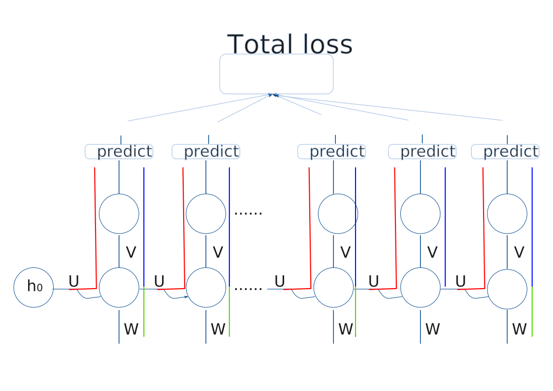
This is backpropagation through time. The algorithm is ordinary backpropagation on the unrolled graph, and the lectures work the three derivatives out in full.

The output matrix is the easy one. With a softmax and cross-entropy the error signal is again prediction minus target:

$$\begin{equation} \frac{\partial E_t}{\partial V} \;=\; \delta_{\text{out}}^{t}\, h_t^{\top}, \qquad \delta_{\text{out}}^{t} \;=\; \hat{y}_t - y_t . \label{eq:bptt-v} \quad\text{(12.2)} \end{equation}$$

The recurrent matrix needs one more link, through the $\tanh$:

$$\begin{equation} \frac{\partial E_t}{\partial U} \;=\; \Big[\big(V^{\top}(\hat{y}_t - y_t)\big) \odot (1 - h_t^2)\Big] h_{t-1}^{\top}, \label{eq:bptt-u} \quad\text{(12.3)} \end{equation}$$

where $\odot$ is elementwise multiplication and $1 - h_t^2$ is the derivative of $\tanh$. The input matrix is identical in form, with $x_t$ in place of $h_{t-1}$:

$$\begin{equation} \frac{\partial E_t}{\partial W} \;=\; \Big[\big(V^{\top}(\hat{y}_t - y_t)\big) \odot (1 - h_t^2)\Big] x_t^{\top}. \label{eq:bptt-w} \quad\text{(12.4)} \end{equation}$$

Because the weights are shared, the gradient for one matrix is the sum of its contributions from every time step. That sum is where the trouble starts.

Why the memory fades

Take an error at step $\tau$ and ask what it says about the state at step $0$. The chain rule gives one factor per step in between:

$$\begin{equation} \frac{\partial E^{[\tau]}}{\partial h^{[0]}} \;=\; \frac{\partial E^{[\tau]}}{\partial h^{[\tau]}} \prod_{t=1}^{\tau} \frac{\partial h^{[t]}}{\partial h^{[t-1]}} . \label{eq:bptt-product} \quad\text{(12.5)} \end{equation}$$

Each factor is a Jacobian, and Equation (12.8) says what it contains:

$$\begin{equation} \frac{\partial h^{[t]}}{\partial h^{[t-1]}} \;=\; \operatorname{diag}\!\big(\tanh'(\cdot)\big)\, U . \label{eq:bptt-jacobian} \quad\text{(12.6)} \end{equation}$$

So the product in Equation (12.5) behaves like $U$ raised to the power $\tau$. The $\tanh$ derivative damps it at each step.

Repeated multiplication by a matrix is governed by its eigenvalues, and the outcome is binary.

If every eigenvalue of $U$ satisfies $|\lambda| < 1$, the product shrinks towards zero. Gradients vanish.

If any eigenvalue satisfies $|\lambda| > 1$, the product grows without bound. Gradients explode.

Only $|\lambda| = 1$ survives, and nothing in training holds it there.

How fast, in numbers

Treat the per-step factor as a single number and raise it to the distance.

Notice how mild the failing factor is. A per-step multiplier of $0.9$ looks harmless, and after fifty steps it has removed more than $99$ per cent of the signal.

The forty-seven word example

The lectures make it concrete. Take this passage.

Raj entered CoffeeDay to meet his partner Dru. Raj said “Hi Dru”. In the next few hours they discussed their start-up and devised a plan to develop a product on knowledge management. After a long and fruitful discussion, Raj said goodbye to his .

The answer is partner, and the evidence sits $47$ words back. Here is what reaches it.

$$0.01^{47} = 1.0 \times 10^{-94}, \qquad 0.5^{47} = 7.1 \times 10^{-15}, \qquad 1.2^{47} = 5266.46 .$$

A gradient of $10^{-94}$ is not a small update. It is no update at all. The weights that would have captured the link never move, so the network cannot learn the dependency however reliably it holds.

One point deserves emphasis, because it is easy to misread. The forward pass is fine. Information does flow from step $1$ to step $47$.

It is the backward pass that fails. The network cannot assign blame across that distance, so it never learns to use the information it is carrying.

Two partial repairs

The two failures are not equally hard, and it is worth being clear about which one has a cheap fix.

Gradient clipping

Exploding gradients have a one line remedy. If the gradient is longer than a threshold, rescale it and keep its direction:

$$\begin{equation} \text{if } \lVert g \rVert > \text{threshold}, \quad g \;\leftarrow\; \frac{\text{threshold}}{\lVert g \rVert}\, g . \label{eq:clipping} \quad\text{(12.7)} \end{equation}$$

The last column is $1$ every time. Clipping changes how far the step goes and never which way it points, which is why it costs nothing in quality.

It does nothing whatever for vanishing gradients. There the problem is that the number is already too small, and scaling it up would amplify noise along with signal.

Truncated backpropagation

Unrolling a sequence of thousands of steps is expensive in memory and slow.

Truncated backpropagation through time splits the sequence into fixed segments and backpropagates within each. A sequence of $5000$ samples becomes $50$ segments of $100$.

The cost is honest and worth stating. Any dependency spanning a segment boundary is invisible to training. Choosing the boundaries at sentence ends reduces the damage without removing it.

Note that truncation is a concession, not a cure. It makes long sequences trainable by giving up on long dependencies, which were the reason for the recurrence in the first place.

Reading both ways

One more variant is worth naming, because it answers a limitation that has nothing to do with gradients.

An RNN reads left to right, so $h_t$ summarises the past and knows nothing of the future. For tagging a word that is often the wrong half of the sentence.

A bidirectional RNN runs two independent recurrences, one forward and one backward. It concatenates their states at each position, so every output sees the whole sentence.

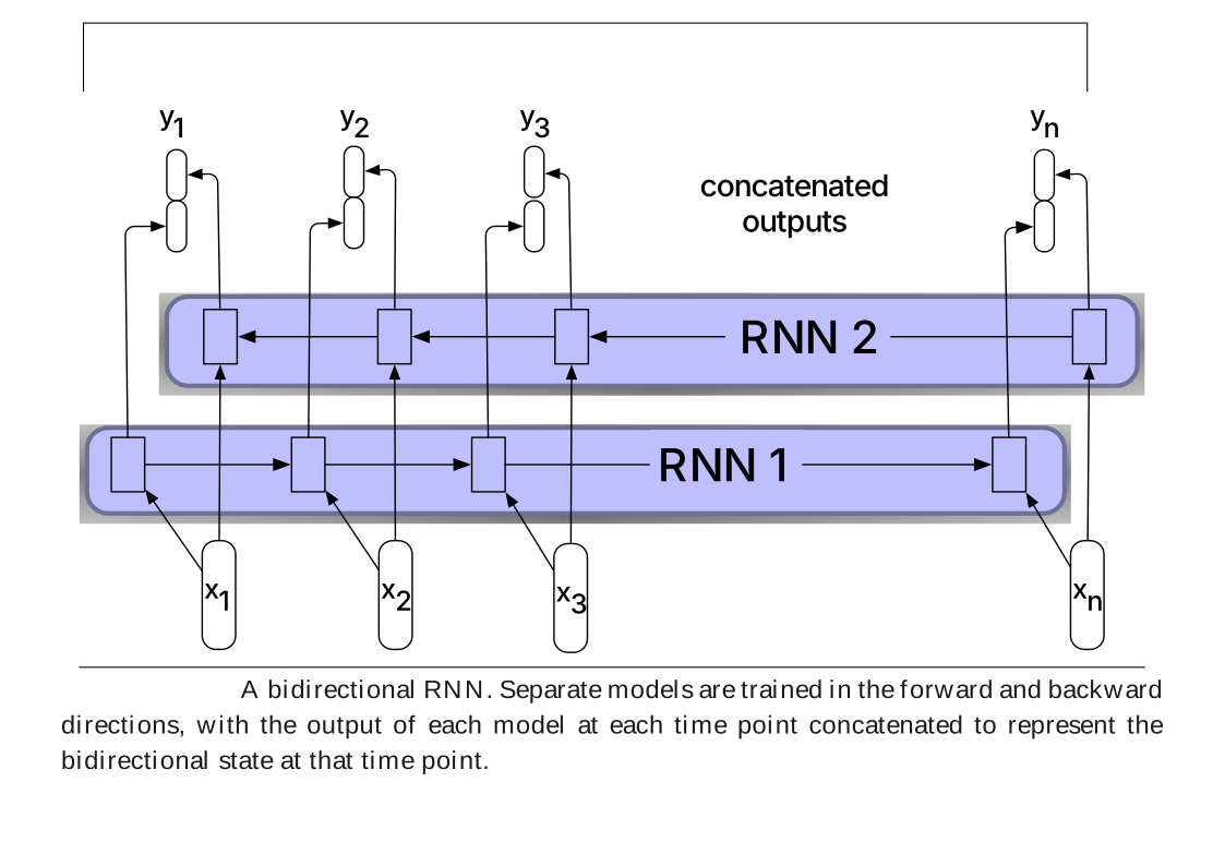
The restriction is obvious once stated. A bidirectional model cannot generate text, because the backward pass would need words that have not been produced yet. It is for labelling, not for prediction.

That distinction returns in Chapter 17, where BERT reads both ways and GPT reads one way, for exactly this reason.

Try it yourself. code/worked_examples/rnn.py produces every table in this chapter. --unroll prints the three step trace, --params the two parameter tables, --vanish the decay table and the forty-seven word arithmetic, and --clip the clipping demonstration with its unchanged directions.

Run it in ColabNotebookSource

What the RNN did and did not buy

The window is gone. State carries an unbounded prefix, and the parameter count no longer depends on sentence length. The same three matrices serve a sentence of any size.

In exchange we inherited a new failure, and it is specific rather than vague. Gradients decay geometrically with distance.

So the network cannot be trained to use information from far back, even though it is perfectly capable of carrying it.

Clipping handles one half. Truncation manages the cost. Neither touches the vanishing case.

The repair has to be architectural. Multiplying by $U$ at every step is what destroys the gradient. So the state needs a path that does not pass through that multiplication.

That path is a gate, and building one is the subject of Chapter 13.

Further reading.

is the original recurrent network for language and remains the clearest short introduction. introduced backpropagation, which backpropagation through time simply applies to an unrolled graph. first proved that gradient descent cannot learn long-term dependencies in this architecture, and analyse both failures and propose clipping. inspect what a trained recurrent network actually stores in its state, and it is unusually readable. shows what these models could already do with sequences.