Chapter 16Self-Attention and the Transformer

The problem attention solves

Part III closed with an evaluation chapter and Part IV opened with a representation one. This chapter picks the architecture thread back up where Chapter 13 put it down.

That chapter ended with two complaints gating could not touch.

The first is sequential computation. A recurrence needs $h_{t-1}$ before it can produce $h_t$, so the time steps cannot run in parallel. That is a hard ceiling, and it arrived precisely when hardware became massively parallel.

The second is the bottleneck. Everything the model knows about the prefix has to fit in one fixed-size vector, however long the prefix is.

Both complaints have one root. Information is forced to travel through the sequence, one step at a time.

So remove the travelling. Let every position look directly at every other position, in one operation, with nothing in between.

Distance stops mattering, because there is no distance any more. And the computation parallelises, because nothing waits for anything.

That is attention.

Where it began

Attention did not arrive with the transformer. It arrived as a patch on a recurrent translation system .

Encoder-decoder translation compressed the whole source sentence into one vector, then decoded from it. Long sentences degraded badly, for the obvious reason.

Bahdanau’s fix let the decoder look back at all the encoder states, and learn a weighting over them at each output step. The bottleneck opened.

The transformer took the next step, and its title says it. Attention was not a patch on recurrence. It could replace it entirely.

Queries, keys, and values

The mechanism borrows its vocabulary from databases, and the analogy is exact enough to be useful.

A query is what a position is looking for. A key advertises what a position offers. A value is what it actually contributes.

In a dictionary lookup you match one query against one key and take that value. Attention is the soft version. Match the query against every key, turn the match scores into weights, and take the weighted average of all the values.

Each of the three is a learned linear projection of the input:

$$\begin{equation} Q = X W^Q, \qquad K = X W^K, \qquad V = X W^V, \label{eq:qkv} \quad\text{(16.1)} \end{equation}$$

where $X$ holds the input vectors, one row per position.

The whole operation is then one line:

$$\begin{equation} \operatorname{Attention}(Q, K, V) \;=\; \operatorname{softmax}\!\left(\frac{Q K^{\top}}{\sqrt{d_k}}\right) V . \label{eq:attention} \quad\text{(16.2)} \end{equation}$$

Read it right to left. $QK^{\top}$ scores every query against every key. Dividing by $\sqrt{d_k}$ keeps those scores in a workable range. The softmax turns each row into a distribution. Multiplying by $V$ takes the weighted average.

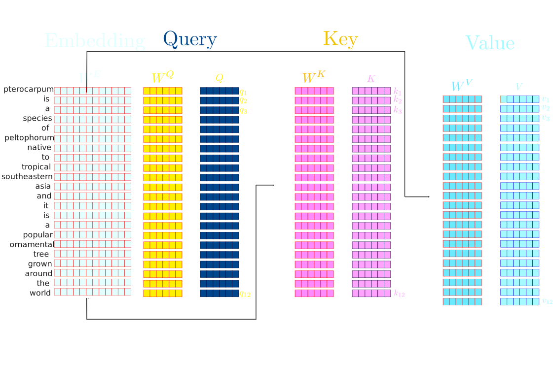
The word self in self-attention means $Q$, $K$ and $V$ all come from the same sequence. Every position queries the sentence it is part of, including itself.

One query, worked

Take the lecture’s example. A query for who, and three keys, in three dimensions. The values equal the keys, to keep the arithmetic short.

$$q = (0.1,\, 0.2,\, 0.3), \qquad k_{\mathit{is}} = (0.4,\, 0.5,\, 0.6), \qquad k_{\mathit{the}} = (0.2,\, 0.1,\, 0.3),$$ $$k_{\mathit{best}} = (0.6,\, 0.7,\, 0.8) .$$

Here $d_k = 3$, so the scale is $\sqrt{3} = 1.7321$.

The output is the weighted sum of the values:

$$\zeta \;=\; 0.3369\,v_{\mathit{is}} + 0.3019\,v_{\mathit{the}} + 0.3611\,v_{\mathit{best}} \;=\; (0.4118,\, 0.4514,\, 0.5816).$$

Now read the $\alpha$ column: $0.34$, $0.30$, $0.36$. That is nearly uniform. Its entropy is $1.5811$ bits against a maximum of $1.5850$.

So this query attended to everything about equally, and the output is close to a plain average. The mechanism ran correctly and selected nothing, because these three keys all point in much the same direction.

That is worth seeing once. Attention is not magic. It selects only when the keys give it something to select on.

Attention that discriminates

Same machinery, keys that disagree. Three dimensions standing for animal, vehicle and verb.

$$k_{\mathit{dog}} = (0.9,\, 0,\, 0.1), \quad k_{\mathit{truck}} = (0,\, 0.9,\, 0.1), \quad k_{\mathit{barked}} = (0.1,\, 0,\, 0.9).$$

The first two queries commit. The third cannot, and its entropy sits exactly at the $1.5850$ bit maximum for three keys.

Entropy is the useful reading here. Low entropy means the head has made a choice. High entropy means it is averaging. Both are legitimate behaviours, and telling them apart is how attention maps get interpreted.

Why divide by $\sqrt{d_k}$

The scale looks arbitrary. It is not, and the reason is measurable.

Let the entries of $q$ and $k$ have unit variance. Their dot product is a sum of $d_k$ terms, so its standard deviation grows like $\sqrt{d_k}$.

Feed larger and larger numbers to a softmax and it saturates. Here is what that does, averaged over 200 random draws with eight keys.

The maximum possible entropy over eight keys is $3$ bits.

Read the raw column. By $d_k = 1024$ the distribution has collapsed onto a single key, which holds $96$ per cent of the weight. This is before any training has happened.

A saturated softmax has almost no gradient. So the head cannot learn its way out of a position it was put in by initialisation alone.

The scaled column barely moves across the whole range. Dividing by $\sqrt{d_k}$ cancels exactly the growth the second column shows. That is why the constant is a square root rather than something tuned.

The causal mask

A language model must not read the future. When predicting the token at position $i$, only positions $j \le i$ may contribute.

Enforce it on the scores, before the softmax:

$$\begin{equation} S_{ij} \;=\; \begin{cases} \dfrac{(QK^{\top})_{ij}}{\sqrt{d_k}}, & j \le i, \\[2ex] -\infty, & j > i . \end{cases} \label{eq:causalmask} \quad\text{(16.3)} \end{equation}$$

Since $e^{-\infty} = 0$, the blocked positions receive exactly zero weight and the surviving ones renormalise to sum to one.

Take four raw scores and apply it.

Every row sums to one, and that is the entire reason the mask goes before the softmax.

Do it the other way, softmax first and then zero the blocked cells, and the rows no longer sum to one.

The first row now sums to $0.4551$. The weight that belonged to the blocked positions has been discarded rather than redistributed.

The damage is worst for the earliest tokens, which have the most future to hide from. Masking first lets the visible positions inherit that weight. Masking second quietly scales the whole row down.

Multiple heads and the rest of the block

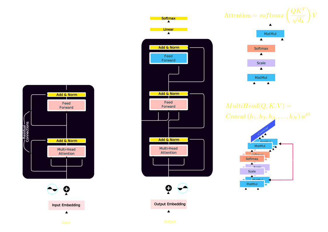
One attention operation computes one kind of relationship. Language has many at once, so run several in parallel.

Multi-head attention splits the model dimension $D$ into $h$ heads of size $d_k = D/h$. Each head runs Equation (16.2) independently. The outputs are concatenated and projected once more with $W^O$.

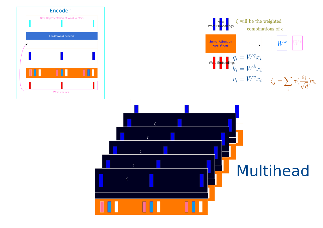
Nobody assigns the heads their jobs. They start from different random initialisations, and specialisation emerges because heads that duplicate each other contribute nothing extra to the loss.

Trained heads are often found tracking recognisable things. Some follow syntactic dependencies, some track the previous token, some resolve coreference. Many appear to do nothing identifiable at all.

The rest of the layer

Attention alone is not a layer. Three more pieces complete it.

A feed-forward network is applied at each position independently. It expands to a larger hidden size, applies a non-linearity, and projects back. This is where most of the layer’s parameters live.

A residual connection adds each sublayer’s input to its output. That gives the gradient a path with no multiplication on it, which is the same repair the LSTM cell state made in Chapter 13.

Layer normalisation rescales each position’s vector to zero mean and unit variance, which keeps the scale stable through a deep stack.

Positional encoding

Equation (16.2) has a property that is easy to miss. It is permutation invariant.

Shuffle the input positions and every attention weight follows them unchanged. The mechanism has no idea which token came first.

That is fatal for language, so position must be added to the input explicitly. The original transformer adds sinusoids of different frequencies:

$$\begin{equation} PE_{(pos, 2i)} = \sin\!\left(\frac{pos}{10000^{2i/D}}\right), \qquad PE_{(pos, 2i+1)} = \cos\!\left(\frac{pos}{10000^{2i/D}}\right). \label{eq:posenc} \quad\text{(16.4)} \end{equation}$$

The frequencies span many scales, so nearby positions get similar encodings and distant ones do not. Later models learn the positional vectors instead, or inject relative position directly into the attention scores.

Counting the parameters

Take the original base configuration. $|V| = 50{,}000$, $D = 512$, $L = 6$ layers, $h = 8$ heads, feed-forward hidden size $H = 2048$.

Two things in that table are worth naming.

The heads are free. Splitting $D$ into eight heads of $64$ costs nothing, because $h \times d_k = D$. Multi-head attention is a reshape, not an extra budget.

The feed-forward block is the larger one, $2.1$ million against $1.0$ million. Attention gets the name and the diagrams, and most of the parameters sit next door.

What the sequence length costs

No entry in that table mentions sequence length. The computation does, because every position attends to every position.

Quadruple the context and the attention cost rises sixteen-fold. That $O(n^2)$ is the price paid for removing the recurrence, and Chapter 23 is largely about paying it down.

Try it yourself. code/worked_examples/attention.py produces every table in this chapter. --one runs the lecture example, --select shows a query that commits and one that cannot, --scale measures the softmax collapsing without the square root, --mask contrasts the two orderings, and --params counts a layer.

Run it in ColabNotebookSource

Why this became everything

Three properties explain the takeover, and only one of them is about quality.

Parallelism. Every position is computed at once. A recurrent network of the same size takes as many sequential steps as there are tokens, and no amount of hardware fixes that.

Constant path length. Any two positions are one attention step apart. In an RNN they are as far apart as the text between them, which is where the gradient died in Chapter 12.

Scale. Because it trains in parallel, it can be made larger, and larger turned out to keep helping for far longer than anyone expected.

Chapter 17 takes this block and builds the two families that followed, one reading in both directions and one reading forwards only.

Further reading.

is the transformer paper, and it is short. introduced attention as a repair to recurrent translation, which is the clearest way to see what problem it solves. is the diagram-led walkthrough most practitioners learn from. cover the same material with more attention to the encoder decoder distinction.